User guide
This page shows how to build PLECS models and Python scripts so that simulations can be automated with plecsutil.
Introduction: basics to create PLECS models, the
model.pyfiles, and running the simulation withplecsutilWorking with controllers: basics to create PLECS models with single or multiple controllers
Saving and loading simulation results: Saving and loading simulation results
Introduction
Creating the PLECS model
To work with plecsutil, the PLECS model needs at least two elements: an output data port in the top-level circuit, and a link to the .m file containing the model parameters.
The output data port (or ports) in the top-level circuit defines which signals are sent to Python at the end of each simulation. A data port can contain a single signal, or many signals can be multiplexed and connected to a single data port. Fig. 1 shows an example of a Buck converter with output data ports in the top-level circuit. (You can download the example by clicking here.)

Fig. 1 PLECS model with output data port in the top-level circuit.
The link to the .m file is given in the initialization tab of the simulation parameters, as shown in Fig. 2. It is important that the name of the .m matches the name of the PLECS model (the simulation file). Thus, if the name of the PLECS model is buck_intro.plecs, the name of the initialization file must be indicated in the simulation parameters must be buck_intro.m.
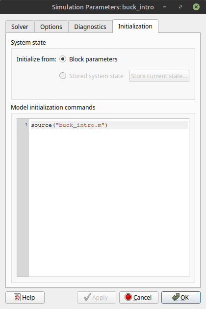
Fig. 2 Initialization of the simulation parameters.
Creating the Python script
Running the PLECS simulation requires creating a plecsutil.ui.PlecsModel object informing the name of the PLECS model, its path, and a Python dictionary containing all of the parameters of the model.
An example of a Python script is shown below. Note that the script assumes to be in the same folder as that the PLECS model, since it defines the plecs_file_path as the current working directory.
import os
import plecsutil as pu
import matplotlib.pyplot as plt
plt.ion()

# Model params
model_params = {
    'f_pwm': 100e3,
    'V_in': 24,
    'R': 10,
    'L': 47e-6,
    'C': 220e-6
    }

# Plecs file
plecs_file = 'buck_intro'
plecs_file_path = os.path.abspath(os.getcwd())

# Plecs model
pm = pu.ui.PlecsModel(plecs_file, plecs_file_path, model_params)

# Runs simulation
data = pm.sim()

# Plots results
plt.figure()
plt.plot(data.t, data.data[:, 1])
In this example, when calling plecsutil.ui.PlecsModel.sim() to run the simulation, plecsutil will generate a .m file. This files contains the model parameters given by the model_params dictionary is used to initialize the plecsutil.ui.PlecsModel object. After generating the .m file, the simulation is launched, which then uses the .m as source.
Simulation results
After running a simulation, plecsutil.ui.PlecsModel.sim() returns a plecsutil.ui.DataSet dataclass holding the simulation results. In addition to the data points, plecsutil.ui.DataSet contains a meta field. This field has a dictionary with a model_params entry that stores the model parameters used to produce the associated simulation results. Thus, the simulation results are always saved with the parameters used to produce them.
Running simulations with different model parameters
The plecsutil.ui.PlecsModel.sim() accepts a sim_params dictionary that can be used to overwrite the default model parameters defined when initializing the plecsutil.ui.PlecsModel object. The sim_params dictionary doesn’t need to contain all model parameters, but just the parameters to be overwritten. In the example Python script shown above, calling plecsutil.ui.PlecsModel.sim() as
data = pm.sim({'R': 4})
will run the simulation with R = 4, instead of the default value of 10 defined by model_params.
An example of running the simulation of the Buck converter with different R values is shown below. In this example, plecsutil.ui.PlecsModel.sim() is called with sim_params specifying different values for R.
import os
import plecsutil as pu
import matplotlib.pyplot as plt
plt.ion()

# Model params
model_params = {
    'f_pwm': 100e3,
    'V_in': 24,
    'R': 10,
    'L': 47e-6,
    'C': 220e-6
    }

# Plecs file
plecs_file = 'buck_intro'
plecs_file_path = os.path.abspath(os.getcwd())

# Plecs model
pm = pu.ui.PlecsModel(plecs_file, plecs_file_path, model_params)

# Runs simulation
R_vals = [2, 5, 10]
data = []
for r in R_vals:
    d = pm.sim(sim_params={'R': r})
    data.append(d)

# Plots results
plt.figure()
for d in data:
    label = 'R = {:}'.format(d.meta['model_params']['R'])
    plt.plot(d.t, d.data[:, 1], label=label)
plt.legend()
The model.py file
In the previous examples, the dictionary containing the model parameters (model_params) was defined in the script that runs the simulation. This makes managing the model parameters more difficult when there are multiple Python scripts to perform different simulations of the same model. In the Buck model used as example, one might create one script to run the model with different values for R, and another one for different values of f_pwm. If the parameters of the PLECS model need to be updated, all scripts need to be modified to include the new parameters.
This can be avoided by creating a model.py associated with the PLECS model. In this way, the model parameters are defined in a single location, and all scripts running simulations can simply import the model from the model.py file.
Although the model.py can be created and define the dictionary with the model parameters, it is more flexible to create a function that returns the parameters instead. The advantages of this approach become clear when adding controllers to the simulation.
For the Buck example discussed thus far, we can create an associated model.py with the following contents:
def params():

    model_params = {
        'f_pwm': 100e3,
        'V_in': 24,
        'R': 10,
        'L': 47e-6,
        'C': 220e-6
        }

    return model_params
Now, model.py can be imported by Python scripts to get the model parameters. For example, to run the Buck converter model with varying values for R:
import os
import plecsutil as pu
import matplotlib.pyplot as plt
plt.ion()

import model

# Plecs file
plecs_file = 'buck_intro'
plecs_file_path = os.path.abspath(os.getcwd())

# Plecs model
pm = pu.ui.PlecsModel(plecs_file, plecs_file_path, model.params())

# Runs simulation
R_vals = [2, 5, 10]
data = []
for r in R_vals:
    d = pm.sim(sim_params={'R': r})
    data.append(d)

# Plots results
plt.figure()
for d in data:
    label = 'R = {:}'.format(d.meta['model_params']['R'])
    plt.plot(d.t, d.data[:, 1], label=label)
plt.legend()
Working with controllers
It is often interesting to see how a closed-loop system behaves, especially when changing controller parameters. There are also case where we have more than one controller and would like to compare them. plecsutil provides a way to define controllers as part of the model, and vary their parameters.
Single controller
When the model has a single controller, changing the parameters of the controller can be done much in the same way as changing the parameters of the model. After all, the controller is part of the model. However, it is often the case that we don’t want to specify the controller gains directly, but rather through some other specifications. For example, we may have a design method, where we specify the settling time of the controller to get the gains. Then, it is a question of concatenating the parameters of the plant with the parameters of the controller, in order to create a single dictionary with all parameters of the model.
Consider state-feedback controller for a Buck converter shown in Fig. 3. This controller has two parameters, which are part of the model parameters: the vector Kx and the gain Ke.

Fig. 3 State-feedback controller for a Buck converter.
These two gains can be determined based on time response specifications of the closed-loop system, such as settling time and overshoot. This is possible with pole placement, based on a model of the converter.
Now, we can identify two sets of parameters: the plant parameters, and the controller parameters. These two combined compose the model parameters. In our model.py file, we can then create three functions: one for the parameters of the plant, one for the parameters of the controller, and one that concatenates them. An example of such structure is shown in the script below.
import numpy as np
import scipy.signal

def plant_params():

    V_in = 20
    Vo_ref = 10

    L = 47e-6
    C_out = 220e-6

    f_pwm = 100e3

    R = 10
    Rd = 10

    params = {}
    params['L'] = L
    params['C_out'] = C_out
    params['R'] = R
    params['Rd'] = Rd

    params['V_in'] = V_in
    params['Vo_ref'] = Vo_ref

    params['f_pwm'] = 100e3

    return params


def controller_gains(ctl_params):

    ts = ctl_params['ts']
    os = ctl_params['os']

    _plant_params = plant_params()
    R = _plant_params['R']
    L = _plant_params['L']
    C = _plant_params['C_out']
    V_in = _plant_params['V_in']

    A = np.array([
        [0,       -1 / L],
        [1 / C,   -1 / R / C]
        ])

    B = np.array([
        [V_in / L],
        [0]
        ])

    C = np.array([0, 1])

    Aa = np.zeros((3,3))
    Aa[:2, :2] = A
    Aa[2, :2] = -C

    Ba = np.zeros((3, 1))
    Ba[:2, 0] = B[:, 0]

    zeta = -np.log(os / 100) / np.sqrt( np.pi**2 + np.log(os / 100)**2 )
    wn = 4 / ts / zeta

    p1 = - zeta * wn + 1j * wn * np.sqrt(1 - zeta**2)
    p2 = np.conj(p1)
    p3 = 5 * p1.real

    K = scipy.signal.place_poles(Aa, Ba, (p1, p2, p3)).gain_matrix

    Kx = K[0, :2]
    Ke = K[0, 2]

    return {'Kx': Kx, 'Ke': Ke}


def params():

    # Plant parameters
    _plant_params = plant_params()

    # Control parameters
    ts = 2e-3
    os = 5
    _ctl_params = controller_gains({'ts':ts, 'os':os})

    # Model params
    _params = {}
    _params.update( _plant_params )
    _params.update( _ctl_params )

    return _params
Note that the controller_gains gain function takes as argument a dictionary, which contains the parameters of the controller. In this case, the parameters are ts (settling time) and os (overshoot). The function also returns a dictionary, containing the gains that are used in the model.
When there is a controller, plecsutil is made aware of it by informing the function that returns the controller gains when creating the plecsutil.ui.PlecsModel object. When running the simulation, the user can set the parameters of the controller and pass them to plecsutil.ui.PlecsModel.sim(). Internally, plecsutil calls the function to get the gains, and updates the parameters of the model automatically. This is demonstrated in the script below.
import os

import plecsutil as pu
import model

import matplotlib.pyplot as plt
plt.ion()

# --- Input ---
plecs_file = 'buck_single_controller'
plecs_file_path = os.path.abspath(os.getcwd())

# --- Sim ---
# Plecs model
pm = pu.ui.PlecsModel(
    plecs_file, plecs_file_path,
    model.params(),
    get_ctl_gains=model.controller_gains
    )

# Runs simulation
data = pm.sim(ctl_params={'ts': 2.5e-3, 'os': 5})

# --- Results ---
plt.figure()
xlim = [0, 20]

ax = plt.subplot(2,1,1)
plt.title('Duty-cycle')
plt.step(data.t / 1e-3, data.data[:, 3], where='post')
plt.grid()
plt.ylabel('$u$')
plt.gca().tick_params(labelbottom=False)

plt.subplot(2,1,2, sharex=ax)
plt.title('Output voltage')
plt.plot(data.t / 1e-3, data.data[:, 1])
plt.grid()
plt.ylabel('Voltage (V)')
plt.xlabel('Time (ms)')
plt.xlim(xlim)

plt.tight_layout()
Note that plecsutil.ui.PlecsModel.sim() is called with ctl_params set to {'ts': 2.5e-3, 'os': 5}. These parameters are used to generate the controller gains, which in turn are updated in the model parameters file.
Now, running the simulation with different controller parameters is just a matter of calling plecsutil.ui.PlecsModel.sim() with different control parameters. An example is demonstrated in the script below.
import os

import plecsutil as pu
import model

import matplotlib.pyplot as plt
plt.ion()

# --- Input ---
plecs_file = 'buck_single_controller'
plecs_file_path = os.path.abspath(os.getcwd())

# --- Sim ---
# Plecs model
pm = pu.ui.PlecsModel(
    plecs_file, plecs_file_path,
    model.params(),
    get_ctl_gains=model.controller_gains
    )

# Runs simulations
data = []
ctl_params = [
    {'ts': 1e-3, 'os': 5},
    {'ts': 3e-3, 'os': 5},
    {'ts': 5e-3, 'os': 5}
    ]
for cp in ctl_params:
    d = pm.sim(ctl_params=cp, close_sim=False)
    data.append(d)

# --- Results ---
plt.figure()
xlim = [0, 20]

ax = plt.subplot(3,1,1)
plt.title('Duty-cycle')
for d in data:
    label = '$T_s = {:}$ ms'.format( d.meta['ctl_params']['ts'] / 1e-3 )
    plt.step(d.t / 1e-3, d.data[:, 3], label=label, where='post')
plt.grid()
plt.ylabel('$u$')
plt.legend()
plt.gca().tick_params(labelbottom=False)

plt.subplot(3,1,2, sharex=ax)
plt.title('Inductor current')
for d in data:
    plt.plot(d.t / 1e-3, d.data[:, 0])
plt.grid()
plt.ylabel('Current (A)')
plt.gca().tick_params(labelbottom=False)

plt.subplot(3,1,3, sharex=ax)
plt.title('Output voltage')
for d in data:
    plt.plot(d.t / 1e-3, d.data[:, 1])
plt.grid()
plt.ylabel('Voltage (V)')
plt.xlabel('Time (ms)')
plt.xlim(xlim)

plt.tight_layout()
Multiple controllers
There are many cases where we would like to have multiple controllers in the model, so that we can easily compare them. This case is also supported in plecsutil, by following a couple of rules in the PLECS model, and by defining the controllers as an plecsutil.ui.Controller object.
First, let’s consider the Buck model we’ve been using so far, and let’s assume we want to compare two controllers: a state feedback and a cascaded controller. First, we define our controller as a configurable subsystem in PLECS, as shown in Fig. 4.

Fig. 4 Buck model with controllers as a configurable subsystem (download model).
Next, we open the configurable subsystem (right-click on subsystem, Subsystem, Open subsystem) and create the controllers there. For this example, we’ve created two subsystems: state_feedback and cascaded, representing the controllers we want to compare. This is shown in Fig. 5.
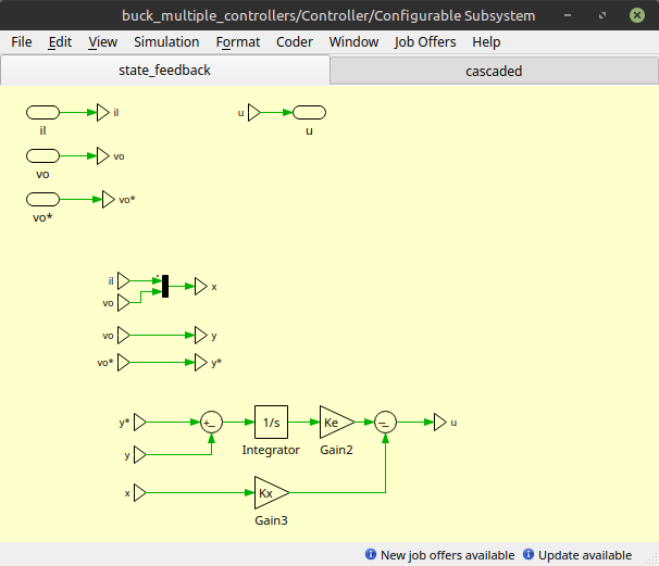
Fig. 5 Controllers in the configurable subsystem.
Now, we go back to the Controller subsystem (Fig. 4), double click on the configurable subsystem containing the controllers, and in the Configuration option we select <reference> and type CTL_SEL, as shown in Fig. 6.
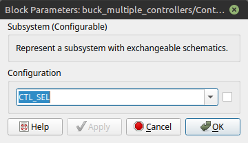
Fig. 6 Setting CTL_SEL as the configuration of the configurable subsystem.
Now, we will build the model.py file much in the same way as before. We can create one function for the parameters of the plant, and one function for each controller. Then, a single function is created to concatenate all the parameters in a single model parameter dictionary. A script for this is shown below.
import numpy as np
import scipy.signal

import plecsutil as pu

def plant_params():

    V_in = 20
    Vo_ref = 10

    L = 47e-6
    C_out = 220e-6

    f_pwm = 100e3

    R = 10
    Rd = 10

    _params = {}
    _params['L'] = L
    _params['C_out'] = C_out
    _params['R'] = R
    _params['Rd'] = Rd

    _params['V_in'] = V_in
    _params['Vo_ref'] = Vo_ref

    _params['f_pwm'] = 100e3

    return _params


def sfb_get_gains(ctl_params):

    ts = ctl_params['ts']
    os = ctl_params['os']

    _plant_params = plant_params()
    R = _plant_params['R']
    L = _plant_params['L']
    C = _plant_params['C_out']
    V_in = _plant_params['V_in']

    A = np.array([
        [0,       -1 / L],
        [1 / C,   -1 / R / C]
        ])

    B = np.array([
        [V_in / L],
        [0]
        ])

    C = np.array([0, 1])

    Aa = np.zeros((3,3))
    Aa[:2, :2] = A
    Aa[2, :2] = -C

    Ba = np.zeros((3, 1))
    Ba[:2, 0] = B[:, 0]

    zeta, wn = _zeta_wn(ts, os)

    p1 = - zeta * wn + 1j * wn * np.sqrt(1 - zeta**2)
    p2 = np.conj(p1)
    p3 = 5 * p1.real

    K = scipy.signal.place_poles(Aa, Ba, (p1, p2, p3)).gain_matrix

    Kx = K[0, :2]
    Ke = K[0, 2]

    return {'Kx': Kx, 'Ke': Ke}


def cascaded_get_gains(ctl_params):

    _plant_params = plant_params()
    R = _plant_params['R']
    L = _plant_params['L']
    C = _plant_params['C_out']
    V_in = _plant_params['V_in']

    ts_v = ctl_params['ts_v']
    os_v = ctl_params['os_v']

    ts_i = ctl_params['ts_i']
    os_i = ctl_params['os_i']

    zeta_i, wn_i = _zeta_wn(ts_i, os_i)
    ki = (L / V_in) * 2 * zeta_i * wn_i
    k_ei = (L / V_in) * ( - wn_i**2 )

    zeta_v, wn_v = _zeta_wn(ts_v, os_v)
    kv = ( C ) * ( 2 * zeta_v * wn_v - 1 / R / C )
    k_ev = ( C ) * ( - wn_v**2 )

    params = {'ki': ki, 'k_ei': k_ei, 'kv': kv, 'k_ev':k_ev}

    return params


def params():

    # Plant parameters
    _plant_params = plant_params()

    # Control parameters
    ts = 2e-3
    os = 5

    _sfb_params = sfb_get_gains({'ts':ts, 'os':os})
    _casc_params = cascaded_get_gains(
        {'ts_v':ts, 'os_v':os, 'ts_i':ts/5, 'os_i':os}
        )

    _ctl_params = {}
    _ctl_params.update( _sfb_params)
    _ctl_params.update( _casc_params)

    # List of controllers
    n_ctl = len(CONTROLLERS)
    active_ctl = 0
    l_ctl = pu.ui.gen_controllers_params(n_ctl, active_ctl)

    # Params for plecs
    _params = {}
    _params.update( _plant_params )
    _params.update( _ctl_params )
    _params.update(l_ctl)

    return _params


def _zeta_wn(ts, os):

    zeta = -np.log(os / 100) / np.sqrt( np.pi**2 + np.log(os / 100)**2 )
    wn = 4 / ts / zeta

    return (zeta, wn)


CONTROLLERS = {
    'sfb' : pu.ui.Controller(idx=1, get_gains=sfb_get_gains, label='State feedback'),
    'casc': pu.ui.Controller(idx=2, get_gains=cascaded_get_gains, label='Cascaded')
}
In the script above, there are two main differences compared to the single controller case. The first one is that the params function includes a call to plecsutil.ui.gen_controllers_params(). This function generates the variable CTL_SEL seen in Fig. 6, which is used to select the controller. The second difference is that at the end of the script, a CONTROLLERS dictionary is defined, containing the two controllers of the model. Each entry of this dictionary contains a label for the controller, and a plecsutil.ui.Controller object initialized with an idx, a get_gains callback, and a label parameter. The value of idx must match the pattern used in the subsystem of the model. In PLECS, subsystems within a configurable subsystem are assigned indices starting at 1 and incrementing from left to right, i.e. state_feedback is index 1, and cascaded is index 2 (see Fig. 5).
Now, we can finally build the script to run the simulations with different controllers, with an example given below. The plecsutil.ui.PlecsModel is created as before, but now we give the controllers of the model with controllers=model.CONTROLLERS. Then, when running the simulation, we give ctl_params just like we do for the single controller models, but we additionally give ctl, which must be one of the controllers defined in model.CONTROLLERS. Note that ctl_params changes for each controller (although they could also be the same).
import os
import plecsutil as pu

import numpy as np

import matplotlib
import matplotlib.pyplot as plt

import model

plt.ion()

# --- Input ---
plecs_file = 'buck_multiple_controllers'
plecs_file_path = os.path.abspath(os.getcwd())

# --- Sim ---
# Plecs model
pm = pu.ui.PlecsModel(
    plecs_file, plecs_file_path,
    model.params(),
    controllers=model.CONTROLLERS
    )

# Runs simulations
d1 = pm.sim(ctl='sfb', ctl_params={'ts':1.5e-3, 'os':5}, save='tst')
d2 = pm.sim(ctl='casc', ctl_params={'ts_v':1.5e-3, 'os_v':5, 'ts_i':0.15e-3, 'os_i':5})
data  = [d1, d2]

# --- Results ---
plt.figure()
xlim = [0, 20]

ax = plt.subplot(2,1,1)
plt.title('Duty-cycle')
for d in data:
    label = '{:}'.format( d.meta['ctl_label'] )
    plt.step(d.t / 1e-3, d.data[:, 3], where='post', label=label)
plt.grid()
plt.ylabel('$u$')
plt.legend()
plt.gca().tick_params(labelbottom=False)

plt.subplot(2,1,2, sharex=ax)
plt.title('Output voltage')
for d in data:
    plt.plot(d.t / 1e-3, d.data[:, 1])
plt.grid()
plt.ylabel('Voltage (V)')
plt.xlabel('Time (ms)')
plt.xlim(xlim)

plt.tight_layout()
Saving and loading simulation results
With plecsutil, it is possible to save and load simulations results. When calling plecsutil.ui.PlecsModel.sim() to run a simulation, it is possible to automatically save the results after a simulation finishes by setting save to a nonempty string. For example, running
pm.sim(ctl='sfb', ctl_params={'ts':1.5e-3, 'os':5}, save='sfb_sim_results', ret_data=False)
will save the simulation results in a file called sfb_sim_results.zip. The data is saved as a plecsutil.ui.DataSet object, which includes simulation and meta data, such as model and controller parameters.
Data is loaded with plecsutil.ui.load_data():
data = pu.ui.load_data('sfb_sim_results')
data is a plecsutil.ui.DataSet object, and can be handled exactly in the same way as simulation results returned by plecsutil.ui.PlecsModel.sim().
Warning
plecsutil uses pickle under the hood for serializing and de-serializing the simulation results. This is simple and efficient, but is not safe for file sharing. Only load simulation data that you generated yourself, or that you trust the source.